This method is useful for comparing two excel or spreadsheets such as .csv files for different values.
If you are familiar with using Excel formulas you shouldn’t have any problems using this method to compare cell data in two spreadsheets.
We use this technique for tasks such as identifying products in an ecommerce store like Magento that need updating to a new value.
The key prerequisite is that the rows in the spreadsheet will need a common unique identifier e.g SKU or ID in the case of product in an ecommerce store.
Step 1 - Identify and prepare the spreadsheets that you would like to compare.
- Identify the spreadsheets that you would like to compare. In this example we are going to use the case of identifying products that have not been updating correctly during a mass import into Magento.
- Export all products from Magento or your selected ecommerce store.
- Get the spreadsheet of data used for the import – where some of the items failed to update and import correctly – save a copy of this with a new file name – we will use this file for comparing the data. For this example we’ll refer to this spreadsheet as Spreadsheet 1.
- Create a copy of the most recent data export as in the point above and then remove the columns from this file that you were not updating and therefore don’t need to be compared. For the rest of the example we’ll refer to this as Spreadsheet 2.
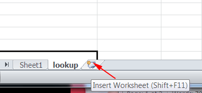
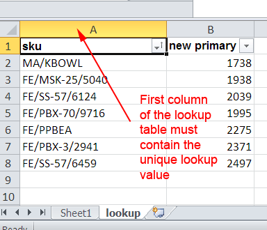
- Create a new worksheet in Spreadsheet 1 and rename the worksheet tab to lookup - and then copy and paste the contents of Spreadsheet 2 into this new worksheet.
6. Make sure that the first column of data being used for the lookup contains the unique identifier for the rows.
7. Save the file.
Step 2 – Add your comparison formula to identify differences
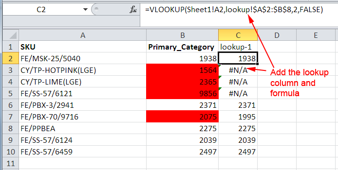
In Spreadsheet 1 add an additional column named lookup-1 or similar – we usually insert this new column next to the column containing the data that we are comparing.
Add a lookup formula to this new column using the vlookup formula that uses the following syntax VLOOKUP(lookup_value, table_array, col_index_num, [range_lookup]), the end result will be along the lines of the following:=VLOOKUP(Sheet1!A2,lookup!$A$2:$B$8,2,FALSE)
To create this use the following steps
i. Type =VLOOKUP(
ii. Select the cell to lookup from and then enter a comma ,
iii. Now click the lookup tab and select all the cells that you are looking up from
iv. Enter a ,
v. Select the number of the column that you are looking up from. In our example we want to obtain the data from the second column so we entered 2 followed by a comma ,
vi. Enter FALSE and close the formula ) - FALSE, means that an exact match lookup will be used which is important for this type of lookup
vii. IMPORTANT: Now add $ in front of each element of cell reference for the lookup table, so that they are fixed references
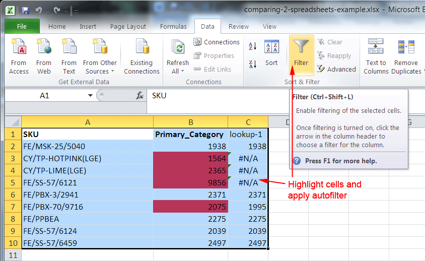
- You should now have a column that contains either the matched lookup value or #N/A – where a match has not been found.
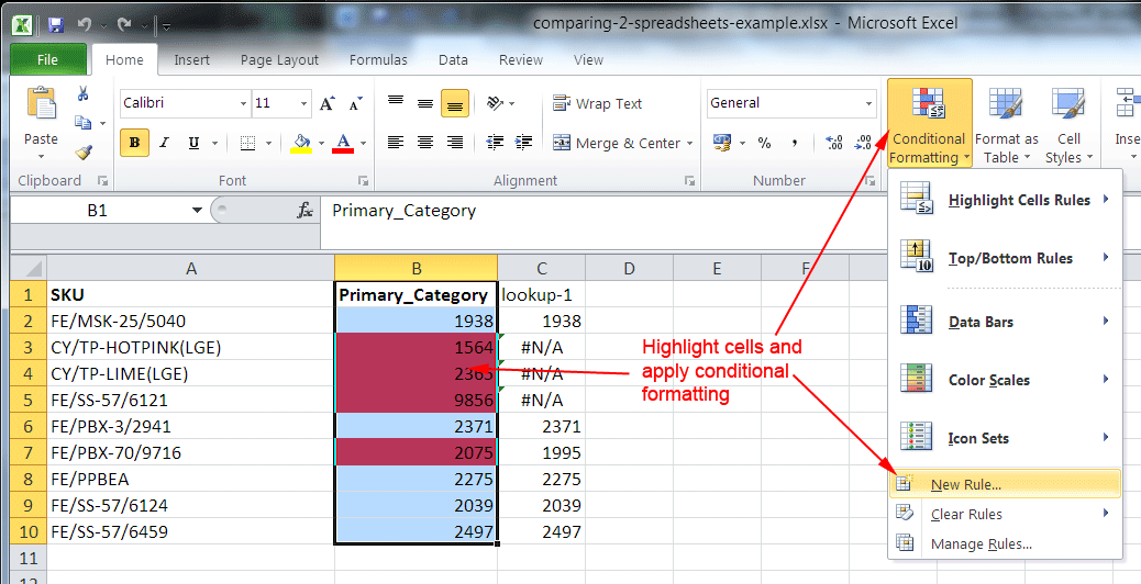
- You can now apply a conditional formatting formula to highlight cells that don’t match
- Highlight the cells that you want highlighted in our example we are highlighting the original cells in column B
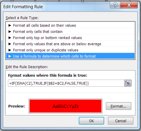
- Select Conditional Formatting > New Rule
3. Select Use a formula to determine which cells to format
4. Enter the following if statement in to the Formula field – updating the cells references as required
i. =IF(ISNA(C2),TRUE,IF($B2=$C2,FALSE,TRUE))
- Select the formatting you would like to apply to the cells e.g. Red background
- Click OK and this should apply the formula (If you have issues with it click manage rules – check the formula is not contained in “” if it is delete the quotation marks – also check the cells that the formula has been applied to the range will always be in for fixed format =$B$2:$B$10)
- You can either sort the spreadsheet or filter it using the Data > Auto Filter functionality and hey presto, you have all the rows that don’t match – which in this example will be the ones that were not correctly updated as part of the Magento import process. Note: If you apply Data > Auto Filter you can sort / filter the spreadsheet by colour.

